Geothermal steam monitoring
Connecting plant signals to a live view of estimated steam quality.
I worked on signal acquisition, model integration, storage, dashboard delivery, and field testing with the research team.
Add a view without replacing the DCS
At Pertamina Geothermal Energy’s Ulubelu facility, installed transmitters already measured steam pressure, temperature, and flow for the Distributed Control System (DCS). Steam dryness followed a slower process: physical sampling and calculation, typically weekly. Our Universitas Padjadjaran research team developed Perta-SMART to provide a live view of the measured signals and a model estimate of dryness between those tests.
I worked on signal acquisition, edge processing, model integration, storage, dashboard delivery, hardware assembly, and testing as an R&D Engineer. Faculty researchers and PGE engineers were part of the project and continued implementation after my part ended. The project was completed in January 2025. My role included integrating the estimator into the monitoring system; I do not claim sole ownership of its training or validation.
Split the signals, preserve the existing route
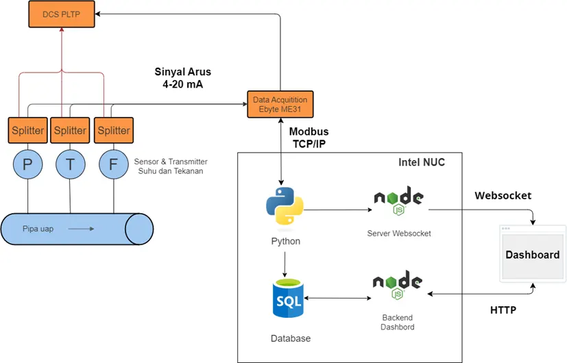
The design kept the existing DCS path in place. Signal splitters supplied a parallel 4–20 mA route from the pressure, temperature, and flow transmitters to an Ebyte ME31 acquisition module. An Intel NUC read that module over Modbus TCP/IP. The Python service scaled raw current readings using configured transmitter ranges before the model and dashboard used them.
Keeping those routes separate mattered in an operating plant. A new web view should not become a hidden dependency for existing control-room instrumentation. Local processing on the NUC also allowed acquisition and estimation to continue when a network connection was unavailable, although remote dashboard access then could not be assumed.
Carry measured signals and an estimate through the system
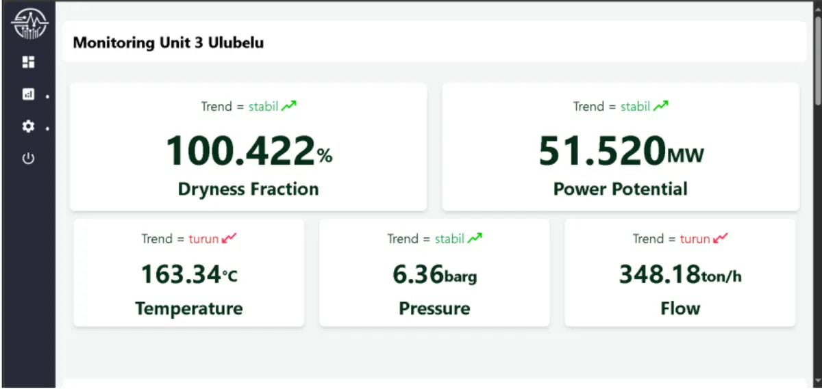
The service passed measured values and the model’s dryness estimate into storage and dashboard paths. PostgreSQL and TimescaleDB held readings and aggregates for later analysis. WebSocket supplied current updates; HTTP served historical queries. The dashboard could show the measured signals beside the estimate, offer filtered histories, and accept physical test results for later model work. That input form does not establish automatic retraining.
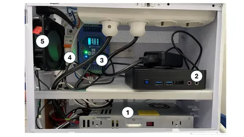
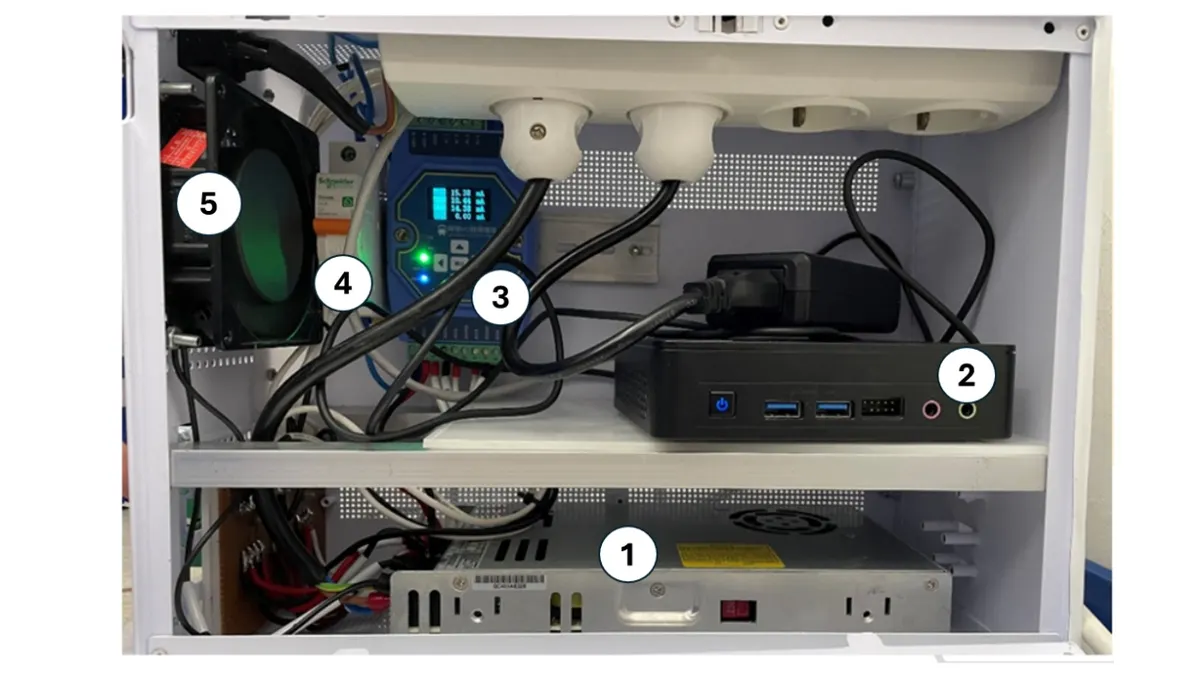
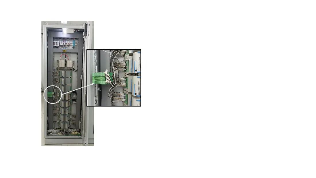
The equipment and wiring had to fit a control-room setting. The enclosure held the NUC and acquisition module; the DCS rack housed the splitter connections. That physical integration was as important to the system as the dashboard route.
The dashboard image in the cover contains demonstration values. It illustrates the interface, not a record of actual plant conditions. Likewise, the model output is an estimate from measured inputs, while periodic physical tests remain the reference measurement.
Read tests within their conditions
The thesis reports laboratory current-loop tests with an average input-path error around 0.048 mA and a largest reported input error of 0.081 mA. Its model plot reports R² = 0.9110 on the plotted evaluation data. R² describes fit in that evaluation; it is not “91.1% accuracy.” The plotted samples’ source and split are unspecified. Controlled service tests with 50 virtual users reported mean delays of 35.047 ms for WebSocket and 232.261 ms for HTTP history. Those figures describe the test conditions, not a plant-wide delivery guarantee.
The work gave the team a parallel signal path, local processing, and a live and historical review interface. My lasting lesson is to keep the provenance of each value visible: measured transmitter signals, a model estimate, and a laboratory reference each answer a different question. For a stronger field evaluation, I would document held-out samples, typical prediction error in dryness percentage points, and how physical tests compare with estimates over time.